Objectives of Inventory

A firm wishing to maximize profit will have at least the following objectives :

- Maximum customer service,
- Improving Operating efficiency by
       - Low-cost plant operation,
       - Minimum inventory investment.

Customer service
In inventory management, the term is used to described the availability of items when needed an is a measure of inventory management effectiveness. Inventories help to maximize customer service by protecting against uncertainty. Demand and lead time to get an item are often uncertain, possible resulting in stockouts and customer dissatisfaction. For these reasons, it may be necessary to carry extra inventory, called safety stock.

Delivering in a Timely Manner : The need to provide quick delivery of goods to users is a primary objective for holding inventories. This is especially true in terms of consumer goods.

Buffering against Uncertainty : Inventories are often held because either the demand for goods or the replenishment of goods is subject to uncertainty. Anticipated demand for products is often forecasted in various ways. Sometimes there is also uncertainty regarding supply; that is, how quickly can goods be replenished? Transportation, quality problems, excessive scrap, and supplier lead times are often
factors contributing to uncertainty for which inventory can compensate.

Providing Variety : Not only is there uncertainty regarding the timing of demand for goods, but there is also uncertainty regarding exactly what will be demanded. This is often the case where goods are available with various options, colors, or packaging. Inventories in a variety of configurations are therefore needed to adequately fulfill customer demands.

Operating efficiency
Inventories help make a manufacturing operation more productive in 4 ways:
- Inventories allow operations with different rates of production to operate separately and more economically;

- To level production, build anticipation inventory for sale in the peak periods. This would result in the following:
o Lower overtime costs,
o Lower hiring and firing costs,
o Lower training costs,
o Lower subcontracting costs,
o Lower capacity required.
By leveling production, manufacturing can continually produce an amount equal to the average demand. The advantage of this strategy is that the costs of changing production levels are avoided;

- Inventories allow manufacturing to run longer production runs, which results in the following:
o Lower setup cost per item. The cost to make a lot depends upon the setups cost and the run costs. The setup costs are fixed, but the run
costs vary with the number produced. If larger lots are run, the setup costs are absorbed over a larger number and the average unit cost is
lower,
o An increase in production capacity due to production resources being used a greater portion of the time for processing as opposed to
setup. If larger quantities are produced at one time, there are fewer setups required to produce a given annual output and thus more
time is available for producing goods. This is most important with bottleneck resources. Time lost on setup on these resources is lost
throughput and lost capacity;

- Inventories allow manufacturing to purchase in larger quantities, which results in lower ordering costs per unit and quantity discounts.

Inv conflict & Resolution
The objectives regarding inventories, indicated above, are often in conflict. Whether used to provide customer service or to achieve efficiencies in procurement or production, inventories conflict with management’s desire to minimize inventory investment. Long production runs by manufacturing operations tend to create large stocks of single products, whereas marketing organizations would often prefer stocks of a larger variety of products and options to serve a broad customer demand.

Large inventories also take up space in factories and distribution centers that is not only expensive to acquire and maintain, but also may lead to loss and confusion as congestion prevents adequate controls and physical storage

The problem is to balance inventory investment with the following:

- Customer service. The higher the inventory level, the higher customer service will be;
- Costs associated with changing production levels. Excess equipment capacity, overtime, hiring, training and layoff costs will be higher if production fluctuates with demand;
- Cost of placing orders. Lower inventories can be achieved by ordering smaller quantities more often, but this practise results in higher annual ordering costs;
- Transportation costs. Goods moved in small quantities cost more to move per unit than those moved in large quantities. However, moving large lots implies higher inventory.

Inventory Control - ABC Analysis & Inv Counting

Control of inventory is exercised by controlling individual items called stockkeeping- units (SKUs). 4 questions must be answered:

- What is the importance of the inventory item?
- How are they to be controlled?
- How much should be ordered at one time?
- When should an order be placed?

The ABC inventory classification system answers the first two questions by determining the importance of items and thus allowing different levels of control based on the relative importance of items.
Usually this is based on annual dollar usage, but other criteria may be used.

The ABC principle is based on Pareto’s law.
As applied to inventories, it is usually found that the relationship between the percentage of items and the percentage of annual dollar usage follows a pattern in which:

- A About 20% of the items account for about 80% of the dollar usage,
- B About 30% of the items account for about 15% of the dollar usage,
- C About 50% of the items account for about 5% of the dollar usage.

This type of distribution can be used to help control inventory.

ABC analysis:
- Establish the items characteristics that influence the results of inventory management,
- Classify items into groups based on the established criteria,
- Apply a degree of control in proportion to the importance of group.

The procedure for classifying by annual dollar usage is as follows:
- Determine the annual usage for each item;
- Multiply the annual usage of each item by its cost to get its total annual dollar usage;
- List the items according to their annual dollar usage;
- Calculate the cumulative annual dollar usage and the cumulative percentage of items;
- Examine the annual usage distribution and group the items into A, B and C groups based on percentage of annual usage.

Control based on ABC classification
Using the ABC approach, there are 2 general rules to follow:
- Have plenty of low-value items. carrying extra stock of C items adds little to the total value of the inventory. C items are really only important if there is a shortage of one of them;
- Use the money and control effort saved to reduce the inventory of highvalue items. A items are extremely important and deserve the tightest control and the most frequent review.

Different controls used with different classifications might be the following:
- A items: high priority. Tight control including complete accurate records, regular and frequent review by management, frequent review of demand forecasts and close follow-up and expediting to reduce lead time;
- B items: medium priority Normal controls with good records, regular attention and normal processing;
- C items: lowest priority Simplest possible control – make sure they are plenty. Simple or no records; perhaps use a two-bin system or periodic review system. Order large quantities and carry safety stock.

Periodic physical counting: are most often performed annually, where all items are counted in a short period of time, often requires shutdown of operations and the use of many diverse personnel. This method does not support day-to-day inventory record accuracy. Its primary purpose is to validate the aggregate inventory values used for financial accounting statements.

Cycle counting: occurs continuously, with a few items, with specified criteria, counted each day by experienced and trained employees. Identification of the trigger for physicalcount activity can be based on one of the following rules:
◊ ABC classification
◊ When a reorder is indicated
◊ When a replenishment lot is received
◊ When the record indicates a zero balance
◊ When a record balance becomes negative
◊ Every specified number of transactions

Fixing Accuracy Targets
Goal of any organization is to achieve 100% inventory accuracy. Practically achieving 100% accuracy target is not easy and can only be achieved over a period of time through cycle counting, where the causes of errors are discovered and corrected. As a practical matter, goals somewhat less that 100% are targeted and might be established based on ABC classification of the inventory items

Order Quantity

In general, when products are demanded on a regular basis (i.e. daily), the logistical problems of getting goods from source of supply to inventory requires that enough goods be ordered in each order cycle to last for some reasonable period of time. The more quantity of goods that are ordered each time, the longer they will last. This is true whether the goods are purchased for resale or manufactured to supply a finished goods warehouse or distribution center.

Graphs shown above contrast two extreme policies to illustrate the range of choices available. The top inventory graph depicts the acquisition of whole year’s supply at one time. The lower graph shows the re-supply policy of one order per week, with 52 orders
placed per year.

In most cases one would conclude that only one order per year is not reasonable because of the space required for the inventory and the cost of buying so much at once. On the other hand 52 orders seems too many with constant authorization and paperwork and excessive receiving and ordering costs. A compromise is called for. But what should it be? Every order quantity decision when done intuitively is based on the comparison of two different costs - the cost to carry the inventory versus the cost to place order.

Economic Order Quantity
All order quantity, or lot-size, choices are based on the principle of economy of scale. It is usually less expensive to purchase (and transport) or produce a bunch of material at once than to order it in small quantities. On other hand, larger lot sizes result in more
inventories and inventory is expensive to hold.

Assumptions
The assumptions on which the EOQ is based are as follows:

- Demand is relatively constant and is known,
- Order preparation costs and inventory-carrying costs are constant and known,
- The items is produced or purchased in lots and not continuously,
- Replacement occurs all at once.

The assumptions are usually valid for finished goods whose demand is independent and fairly uniform. However, there are many situations where the assumptions are not valid (e.g. made-to-order items, shelf life of the product is short,…). In MRP, the lot-for-lot decision rule is often used, but there are also several rules that are variations of the EOQ.

Development of the EOQ formula
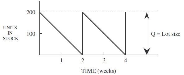
Under the assumptions given, the quantity of an item in inventory decreases at a uniform rate. The vertical lines represent stock arriving all at once as the stock on hand reaches zero. The quantity of units in inventory then increases instantaneously by Q, the quantity ordered.

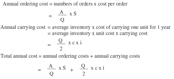
Average lot size inventory = (Order quantity)/ 2
Number of order per year = Annual demand / Order quantity
the number of order per year is rounded neither up nor down.

Relevant costs
The relevant cost are as follows:
- Annual cost of placing orders,
- Annual cost of carrying inventory.
As the order quantities increases, the average inventory and the annual cost of carrying inventory increase, but the number of orders per year and the ordering cost decrease. The trick is to find the particular order quantity in which the total cost of carrying inventory and the cost of ordering will be a minimum.
A = annual usage in units
S = ordering cost in dollar per order
i = annual carrying cost rate as a decimal of a percentage
c = unit cost in dollars
Q = order quantity in units

Ideally, the total cost will be a minimum. For any situation in which the annual demand (A), the cost of ordering (S) and the cost of carrying inventory (i) are given, the total cost will depend upon the order quantity (Q).

Economic-order quantity formula
The EOQ occurred at an order quantity in which the ordering costs equal the carrying costs.
Carrying costs = ordering costs

EOQ MODEL Variation

There are several modifications that can be made to the basic EOQ model to fit particular circumstances. 2 that are often used are the monetary unti to lot-size model and the noninstantaneous receipt model.

Monetary unit lot size
The EOQ can be calculated in monetary units rather than physical units. The same EOQ formula given can be used with:
Ad = annual usage in dollars
S = ordering cost in dollars
I = carrying cost rate as a decimal of a percent


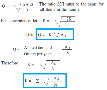
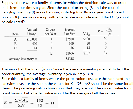
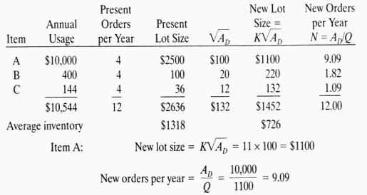
EOQ when costs are unknown
The EOQ formula depends upon the cost of ordering and the cost of carrying inventory. In practise, these costs are not necessarily known or easy to determine.
For a family of items, the ordering costs (S) and the carrying costs (c) are generally the same for each item.

Quantity Discount
When material is purchased, suppliers often give a discount on orders over a certain size. The buyer must decide whether to accept the discount and, in doing so, must consider the relevant costs:
- Purchase cost,
- Ordering costs,
- Carrying costs.

It can be said that taking the discount results in the following:
- There is a saving in purchase cost,
- Ordering costs are reduced because fewer orders are placed since larger quantities are being ordered,
- Inventory –carrying costs rise because of the larger order quantity.
The buyer must weigh the first 2 against the last and decide what to do. What count is the total cost. Depending on the figures, it may or may not be best to take the discount.

Period Order Quantity

The EOQ attempts to minimize the total cost of ordering and carrying inventory and is based on the assumption that demand is uniform. Often demand is not uniform, particularly in MRP and using the EOQ does not produce a minimum cost. The period order quantity lot-size rule is based on the same theory as the EOQ. It uses the EOQ formula to calculate an economic time between orders. This is calculated by dividing the EOQ by the demand rate. This produce a time interval for which orders are placed. Instead of ordering the same quantity (EOQ), orders are placed to satisfy requirements for the calculated time interval. The number of orders placed in a year is the same as for an EOQ, but the amount ordered each time varies. Thus, the ordering cost is the same but , because the order quantities are determined by actual demand, the carrying cost is reduced.

Period-order quantity = EOQ / Average weekly usage

Practical considerations when using the EOQ

Lumpy demand
The EOQ assumes that demand is uniform and replenishment occurs all at once. When this is not true, the EOQ will not produce the best results. It is better to use the period-order quantity.

Anticipation inventory
Demand is not uniform and stock must be built ahead. It is better to plan a buildup of inventory based on capacity and future demand.

Minimum order
Some suppliers require a minimum order. This minimum may be based on the total order rather than an individual items. often these are C items where the rule is to order plenty, not an EOQ.

Transportation inventory
Carriers give rates based on the amount shipped. A full load costs less per ton to ship than a part load. This is similar to the price break
given by suppliers for large quantities. The same type of analysis can be used.

Multiples
Sometimes, order size is constrained by package size. In these case, the unit used should be the minimum package size.

Periodic Review System
Using the periodic review system, the quantity ordered is usually predetermined at specified, fixed-time intervals and an order is placed. Thus the review period is fixed and the order quantity is allowed to vary. The quantity on hand plus the quantity ordered must be sufficient to last until the next shipment is received.

That is, the quantity on hand plus the quantity ordered must equal the sum of the demand during the lead time plus the demand during the review period plus the safety stock.
This sum of quantities is called the target level or maximum-level inventory:

T = D(R + L) + SS
Where
T = Target (maximum) level inventory,
D = Demand per unit of time,
L = Lead-time duration,
R = Review period duration,
SS = Safety stock.
The order quantity (Q) is equal to the maximum-inventory level (T) minus the quantity on hand (I) at the review period:
Q = T – I

The periodic review system is useful for the following:
- Where there are many small issues from inventory and posting transactions to inventory records are very expensive. Supermarkets and retailers are in this category.
- Where ordering costs are small. This occurs when many different items are ordered from the one source. A regional distribution center may order most of all of its stock from a central warehouse.
- Where many items are ordered together to make up a production run or fill a truckload. A good example of this regional distribution center that orders a truckload once a week from a central warehouse.

Order Point System

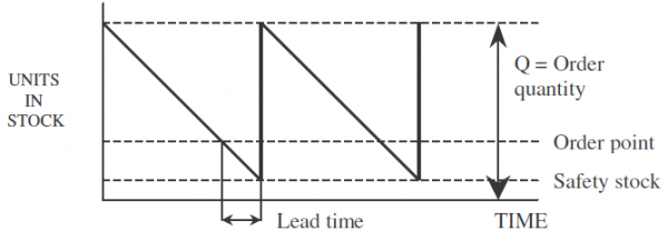
When the quantity of an item on hand in inventory falls to a predetermined level, called an order point, an order is placed. The quantity ordered is usually precalculated and based on economic-order-quantity concepts.

Using this system, an order must be placed when there is enough stock on hand to satisfy demand from the time the order is placed until the new stock arrives (called the lead time). Demand during any one lead-time period probably varies from the average demand. Statistically, half the time the demand is greater than average and there is stockout. If it necessary to provide some protection against stockout, safety
stock can be added. The item is ordered when the quantity on hand falls to a level equal to the demand during the lead time plus the safety stock:

OP = DDLT + SS
OP = order point, DDLT = demand during lead time, SS = safety stock

Figure shows the relationship between safety stock, lead time, order quantity and order point. With the order point:
- Order quantities are usually fixed;
- The order point is determined by the average demand during the lead time. If the average change in the order point, effectively there has been a change in safety stock;
- The intervals between replenishment are not constant but vary depending on the actual demand during the reorder cycle;
- Average inventory = order quantity/2 + safety stock = Q/2 + SS.

Safety Stock Calculations

Safety stock is intended to protect against uncertainty in supply and demand. Uncertainty may occur in 2 ways: quantity uncertainty and timing uncertainty. Quantity uncertainty occurs when the amount of supply and demand varies. Timing uncertainty occurs when the time of receipt of supply or demand differs from than expected.

Two common methods to determine the size of the safety stock are the availability method and the service level method. The desired availability (denoted as AV) becomes AV = probability of not running out of stock during the lead time. The desired service level (denoted as SL) is typically measured as SL = (demand filled) over (total demand). The safety stock is the stock carried to meet the uncertainty associated with the forecasts of the demands.

The difficulty in the above statements is that oftentimes it is confusing which method is being applied to generate the safety stock. The term service level is the most common, followed perhaps by availability and percent fill. In the above definitions, the measure of availability is a probability and the measure of service level is a ratio falling between zero and one. Although both methods of finding the safety stock yield different results -- it is noted in many references -- the term service level is often the only term used for both of the methods. That is, the definition given above for availability is often referred as the service level. Sometimes the term percent fill is used in place of the service level. For convenience in this paper, the terms availability and service level are used in the following way:

availability = probability of (not out of stock during the lead time)
service level = ratio of (demand filled / total demand)

There are 2 ways to protect against uncertainty: carry extra stock, called safety stock, or order earlier, called safety lead time. Both result in extra inventory, but the methods of calculation are different. Safety stock is the most common way of buffering. The SS required depends on the following:
- variability of demand during the lead time;
- frequency of reorder;
- service level desired;
- length of a lead time. The longer the lead time, the more safety stock has to be carried to provide a specified service level. This is one reason it is important to reduce lead time.

Variation in demand during lead time
Actual demand varies from forecast for 2 reasons: bias error in forecasting the average demand and random variations in demand about average. It is the latter with which we are concerned in determining safety stock. Some method of estimating the randomness of item demand is needed.

Variation in demand about the average
Suppose a history of weekly demand for a particular item shows an average demand. As expected, most of the demand are around it. A smaller number would be farther away from it and still fewer would be farthest away. If the weekly demands are classified into groups or ranges about the average , a picture of the distribution of demand about the average appears.

Normal distribution

The pattern of demand distribution about the average will differ for different products and markets. Some method is needed to described the distribution: its shape, center and spread. As long as the demand conditions remain the same, we can expect the pattern to remain very much the same. If the demand is
erratic, so is, the demand pattern, making it difficult to predict with any accuracy.

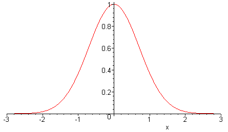
The most common predictable pattern is called a normal curve or bell curve. The normal distribution has most of the value s clustered near a central point with progressively fewer results occurring away from the center. It is symmetrical about this central point in that is spreads out evenly on both sides.
The normal curve is described by 2 characteristics. One relates to its central tendency, the average, and the other to the variation, or dispersion, of the actual values about the average.

Average or mean
The average or mean value is at the high point of the curve. It is the central tendency of the distribution. The symbol is x. It is calculated by adding the data Sum(x) and dividing by the total number of data (n).
x = Sum(x) / n

Dispersion
The variation, or dispersion, of actual demands about the average refers to how closely the individual values cluster around the mean. It can be measure in several ways:
- As a range of the maximum minus the minimum value;
- As the mean absolute deviation (MAD), which is a measure of the average forecast error;
- As a standard deviation.

Standard deviation (sigma)
The standard deviation is a statistical value that measures how closely the individual values cluster about the average. It is represented by s. It is calculated as follows:
- Calculate the deviation for each period by subtracting the actual demand from the forecast demand;
- Square each deviation;
- Add the squares of the deviations;
- Divide the value in previous step by the number of periods to determine the average of squared deviations;
- Calculate the square root of the value calculated in the previous step. This is the standard deviation.
It is important to note that the deviations in demand are for the same timeintervals as the lead time.
From statistics, we can determine that:

- The actual demand will be within ± 1s of the forecast average approximately 68% of the time,
- The actual demand will be within ± 2s of the forecast average approximately 98% of the time,
- The actual demand will be within ± 3s of the forecast average approximately 99.88% of the time.

Determining the safety stock and order point
One property of the normal curve is that is symmetrical about the average.
Safety stocks are needed to cover only those periods in which the demand during the lead time is greater than the average. Thus, a service level of 50% can be attained with no safety stock.

As stated earlier, we know from statistics that the error is within ± 1s of the forecast about 68% of the time. Suppose the standard deviation of demand during the lead time is 100 units and this amount is carried as safety stock. This much safety stock provides protection against stockout for 34% of the time that actual demand is greater than expected. In total, there is enough safety stock to provide protection for the 84% of the time (50% + 34%) that a stockout is possible. The service level is a statement of the percentage of time

The service level is a statement of the percentage of time there is no stockout. It means being able to supply when a stockout is possible and a stockout is possible only at the time an order is to be placed.

Safety factor

The service level is directly related to the number of standard deviation provided as a safety stock and is usually called the safety factor. Note that the service level is the percentage of order cycles without a stockout.

Changing Safety Stock

Records of actual demand and forecasts are normally made on a weekly or monthly basis for all items regardless of what the individual lead times are. It is impossible to measure the variation in demand about average for each of the lead times. Some method of adjusting standard deviation for the different time intervals is needed.

As the lead times increases, the standard deviation increases. However, it will not increase in direct proportion. As the time interval increases, there is a smoothing effect, and the longer the time interval, the more smoothing take place. The following adjustment can be made to the standard deviation or the safety
stock to compensate for differences between lead-time interval (LTI) and forecast interval (FI). While not exact, the formula gives a good approximation:

Order Point Determination

There must be some method to show when the quantity of an item on hand has  reached the order point. There are many systems, but they all are inclined to be variations or extensions of 2 basic systems: the two-bin system and the perpetual inventory system.

Two-bin system

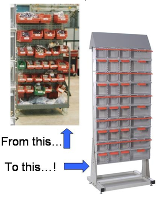
A quantity of an item equal to the order point quantity is set aside and not touched until all the main stock is used up. When this stock needs to be used, the production control or purchasing department is notified and a replenishment order is placed.

The two-bin system is a simple way of keeping control of C items. Because they are of low value, it is best to spend the minimum amount of time and money controlling them. However, they do need to be managed. When it is out of stock, C item becomes an A item.

Perpetual inventory record system
A perpetual inventory record is a continual account of inventory transaction as they occur. At any instant, it holds an up-to-date record of transactions. At a minimum, it contains the balance on hand, but it may also contain the quantity on order but not received, the quantity allocated but not issue and the available balance.

Permanent information is shown at the top of figure. Although not absolutely permanent, this information does not change frequently. It includes data as follows:
- Part number, name, and description;
- Storage location;
- Order point;
- Order quantity;
- Lead time;
- Safety stock;
- Suppliers.

Variable information is information that changes with each transaction and includes the following:
- Quantities ordered: data, order numbers and quantities;
- Quantities received: data, order numbers and quantities;
- Quantities issued: data, order numbers and quantities;
- Balance on hand;
- Quantities allocated: data, order numbers and quantities;
- Available balance.
The information depends of the needs of company and the particular circumstances.