Exponential Smoothing

It is not necessary to keep months of history to get a moving average. Therefore, the forecast can be based on the old calculated forecast and the new data. This formula puts as much weight on the most recent month as on the old average. If this does not seem suitable, less weight could be put on the latest actual demand and more weight on the old forecast. One advantage to exponential smoothing is that the
new data can be given any weight wanted. The weight given to latest demand is called a smoothing constant (a). It is always expressed as a decimal from 0 to 1.0. 
                                        New forecast = (a) (latest demand) + (1 - a) (previous forecast)

Example
The old forecast for May was 220, and the actual demand for May was 190. If alpha (a) is 0.15, calculate the forecast for June. If June demand turns out to be 218, calculate the forecast for July.

Answer
June forecast = (0.15)(190) + (1 — 0.15)(220) = 215.5
July forecast = (0.15)(218) + (0.85)(215.5) = 215.9

Exponential smoothing provides a routine method for regularly updating item forecasts. It works quite well when dealing with stable items. Generally, it has been found satisfactory for short-range forecasting. It is not satisfactory where the demand is low or intermittent.

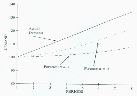
Exponential smoothing will detect trends, although the forecast will lag actual demand if a definite trend exists. The above figure shows a graph of the exponentially smoothed forecast lagging the actual demand where a positive trend exists. Notice the forecast with the larger a follows actual demand more closely.

If a trend exists, it is possible to use a slightly more complex formula called double exponential smoothing. This technique uses the same principles but notes whether each successive value of the forecast is moving up or down on a trend line. Double exponential smoothing is beyond the scope of this text.

A problem exists in selecting the “best” alpha factor. If a low factor such as 0.1 is used, the old forecast will be heavily weighted, and changing trends will not be picked up as quickly as might be desired. If a larger factor such as 0.4 is used, the forecast will react sharply to changes in demand and will be erratic if there is a sizable random fluctuation. A good way to get the best alpha factor is to use computer simulation. Using past actual demand, forecasts are made with different alpha factors to see which one best suits the historical demand pattern for particular products.